Version: 8.3.0
For fields with polynomial representation on each cell, the components of the discretized field  on the source side can be expressed as linear combinations of the components of the discretized field
  on the target side, in terms of a matrix-vector product:
![\[ \phi_t=W.\phi_s. \]](form_13.png)
 is called theinterpolation matrix. The objective of interpolators is to compute the matrix W depending on their physical properties (Overview: intensive and extensive field) and their mesh discretization (on cells P0, on nodes P1,...).
At the basis of many CFD numerical schemes is the fact that physical quantities such as density, momentum per unit volume or energy per unit volume obey some balance laws that should be preserved at the discrete level on every cell.
It is therefore often desired that the process interpolation preserve the integral of  on any domain. At the discrete level, for any target cell
  , the following general interpolation formula has to be satisfied :
![\[ \int_{T_i} \phi_t = \sum_{S_j\cap T_i \neq \emptyset} \int_{T_i\cap S_j} \phi_s. \]](form_17.png)
This equation is used to compute  , based on the fields representation ( P0, P1, P1d etc..) and the geometry of source and target mesh cells.
Another important property of the interpolation process is the maximum principle: the field values resulting from the interpolation should remain between the upper and lower bounds of the original field. When interpolation is performed between a source mesh S and a target mesh T the aspect of overlapping is important. In fact if any cell of of S is fully overlapped by cells of T and inversely any cell of T is fully overlapped by cells of S that is
![\[ \sum_{S_j} Vol(T_i\cap S_j) = Vol(T_i),\hspace{1cm} and \hspace{1cm} \sum_{T_i} Vol(S_j\cap T_i) = Vol(S_j) \]](form_19.png)
then the meshes S and T are said to be overlapping. In this case the two formulas in a given column in the table below give the same result. All intensive formulas result in the same output, and all the extensive formulas give also the same output.
The ideal interpolation algorithm should be conservative and respect the maximum principle. However such an algorithm can be impossible to design if the two meshes do not overlap. When the meshes do not overlap, using either  or
or  one obtains an algorithm that respects either the conservativity or the maximum principle (see the nature of field summary table).
We assume that the field is represented by a vector with a discrete value on each cell. This value can represent either
For intensive fields such as mass density or power density, the left hand side in the general interpolation equation becomes :
![\[ \int_{T_i} \phi = Vol(T_i).\phi_{T_i}. \]](form_22.png)
Here Vol represents the volume when the mesh dimension is equal to 3, the area when mesh dimension is equal to 2, and length when mesh dimension is equal to 1.
In the general interpolation equation the right hand side becomes :
![\[ \sum_{S_j\cap T_i \neq \emptyset} \int_{T_i\cap S_j} \phi = \sum_{S_j\cap T_i \neq \emptyset} {Vol(T_i\cap S_j)}.\phi_{S_j}. \]](form_23.png)
As the field values are constant on each cell, the coefficients of the linear remapping matrix  are given by the formula :
![\[ W_{ij}=\frac{Vol(T_i\cap S_j)}{ Vol(T_i) }. \]](form_25.png)
In code coupling from neutronics to hydraulics, extensive field of power is exchanged and the total power should remain the same. The discrete values of the field represent the total power contained in the cell. Hence in the general interpolation equation the left hand side becomes :
![\[ \int_{T_i} \phi = P_{T_i}, \]](form_26.png)
while the right hand side is now :
![\[ \sum_{S_j\cap T_i \neq \emptyset} \int_{T_i\cap S_j} \phi = \sum_{S_j\cap T_i \neq \emptyset} \frac{Vol(T_i\cap S_j)}{ Vol(S_j)}.P_{S_j}. \]](form_27.png)
The coefficients of the linear remapping matrix are then given by the formula :
![\[ W_{ij}=\frac{Vol(T_i\cap S_j)}{ Vol(S_j) }. \]](form_28.png)
In the case of fields with a P0 representation (cell based) and when the meshes do not overlap, the scheme is either conservative or maximum preserving (not both). Depending on the Nature of a field the interpolation coefficients take the following value:
| Intensive | extensive | |
| Conservation |
IntensiveConservation |
ExtensiveConservation |
| Maximum principle |
IntensiveMaximum |
ExtensiveMaximum |
Let's consider the following case with a source mesh containing two cells and a target mesh containing one cell. Let's consider a field FS on cells on the source mesh that we want to interpolate on the target mesh.
The value of FS on the cell#0 is 4 and the value on the cell#1 is 100.
The aim here is to compute the interpolated field FT on the target mesh of field FS depending on the nature of the field.
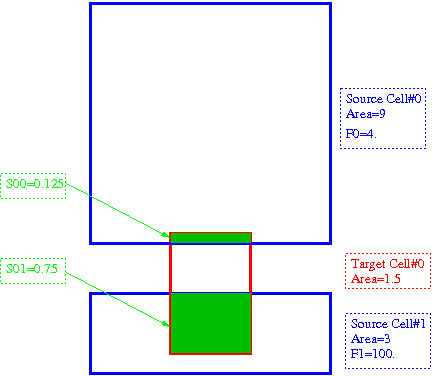
The first step of the interpolation leads to the following M1 matrix :
![\[ M1=\left[\begin{tabular}{cc} 0.125 & 0.75 \\ \end{tabular}\right] \]](form_33.png)
If we apply the formula above it leads to the following  matrix :
![\[ M_{Conservative Volumic}=\left[\begin{tabular}{cc} $\displaystyle{\frac{0.125}{0.125+0.75}}$ & $\displaystyle{\frac{0.75}{0.125+0.75}}$ \\ \end{tabular}\right]=\left[\begin{tabular}{cc} 0.14286 & 0.85714 \\ \end{tabular}\right] \]](form_35.png)
![\[ FT=\left[\begin{tabular}{cc} $\displaystyle\frac{0.125}{0.875}$ & $\displaystyle\frac{0.75}{0.875}$ \\ \end{tabular}\right].\left[\begin{tabular}{c} 4 \\ 100 \\ \end{tabular}\right] =\left[\begin{tabular}{c} 86.28571\\ \end{tabular}\right] \]](form_36.png)
As we can see here the maximum principle is respected.This nature of field is particularly recommended to interpolate an intensive field such as temperature or pressure.
If we apply the formula above it leads to the following  matrix :
![\[ M_{ExtensiveMaximum}=\left[\begin{tabular}{cc} $\displaystyle{\frac{0.125}{9}}$ & $\displaystyle{\frac{0.75}{3}}$ \\ \end{tabular}\right]=\left[\begin{tabular}{cc} 0.013888 & 0.25 \\ \end{tabular}\right] \]](form_38.png)
![\[ FT=\left[\begin{tabular}{cc} $\displaystyle{\frac{0.125}{9}}$ & $\displaystyle{\frac{0.75}{3}}$ \\ \end{tabular}\right].\left[\begin{tabular}{c} 4 \\ 100 \\ \end{tabular}\right] =\left[\begin{tabular}{c} 25.055\\ \end{tabular}\right] \]](form_39.png)
This type of interpolation is typically recommended for the interpolation of power (NOT power density !) for a user who wants to conserve the quantity only on the intersecting part of the source mesh (the green part on the example)
This type of interpolation is equivalent to the computation of  followed by a multiplication by
  where is given by :
![\[ FS_{vol}=\left[\begin{tabular}{c} $\displaystyle{\frac{4}{9}}$ \\ $\displaystyle{\frac{100}{3}}$ \\ \end{tabular}\right] \]](form_42.png)
In the particular case treated here, it means that only a power of 25.055 W is intercepted by the target cell !
So from the 104 W of the source field  , only 25.055 W are transmitted in the target field using this nature of field. In order to treat differently a power field, another policy, integral global constraint nature is available.
If we apply the formula above it leads to the following  matrix :
![\[ M_{ExtensiveConservation}=\left[\begin{tabular}{cc} $\displaystyle{\frac{0.125}{0.125}}$ & ${\displaystyle\frac{0.75}{0.75}}$ \\ \end{tabular}\right]=\left[\begin{tabular}{cc} 1 & 1 \\ \end{tabular}\right] \]](form_45.png)
![\[ FT=\left[\begin{tabular}{cc} 1 & 1 \\ \end{tabular}\right].\left[\begin{tabular}{c} 4 \\ 100 \\ \end{tabular}\right] =\left[\begin{tabular}{c} 104\\ \end{tabular}\right] \]](form_46.png)
This type of interpolation is typically recommended for the interpolation of power (NOT power density !) for a user who wants to conserve all the power in its source field. Here we have 104 W in source field, we have 104 W too, in the output target interpolated field.
BUT, As we can see here, the maximum principle is not respected here, because the target cell #0 has a value higher than the two intercepted source cells.
If we apply the formula above it leads to the following  matrix :
![\[ M_{IntensiveConservation}=\left[\begin{tabular}{cc} $\displaystyle{\frac{0.125}{1.5}}$ & $\displaystyle{\frac{0.75}{1.5}}$ \\ \end{tabular}\right]=\left[\begin{tabular}{cc} 0.083333 & 0.5 \\ \end{tabular}\right] \]](form_48.png)
![\[ FT=\left[\begin{tabular}{cc} $\displaystyle{\frac{0.125}{1.5}}$ & $\displaystyle{\frac{0.75}{1.5}}$ \\ \end{tabular}\right].\left[\begin{tabular}{c} 4 \\ 100 \\ \end{tabular}\right] =\left[\begin{tabular}{c} 50.333\\ \end{tabular}\right] \]](form_49.png)
This type of nature is particulary recommended to interpolate an intensive density field (moderator density, power density). The difference with conservative volumic seen above is that here the target field is homogenized to the whole target cell. It explains why this nature of field does not follow the maximum principle.
To illustrate the case, let's consider that is a power density field in  . With this nature of field the target cell #0 accumulates 0.125*4=0.5 W of power from the source cell #0 and 0.75*100=75 W of power from the source cell #1. It leads to 75.5 W of power on the whole target cell #0. So, the final power density is equal to 75.5/1.5=50.333 W/m^2.


![\[\frac{Vol(T_i\cap S_j)}{ Vol(T_i)}\]](form_29.png)
![\[ \frac{Vol(T_i\cap S_j)}{ \sum_{T_i} Vol(S_j\cap T_i) }\]](form_30.png)
![\[\frac{Vol(T_i\cap S_j)}{ \sum_{S_j} Vol(T_i\cap S_j)}\]](form_31.png)
![\[\frac{Vol(T_i\cap S_j)}{ Vol(S_j) }\]](form_32.png)