Like other intersectors the aim of this intersector is to compute intersection between 2 polygons.
The specificity of this intersector is to deal with any type of polygons even those with quadratic edges. Its quite generic architecture allows him to deal with some other potentially useful functions.
This page described Geometric2D intersector basic principles and specific usage.

Introduction

The principle used in this intersector to perform boolean operation on geometry is geometric-modeler like. The data structure used to describe polygons is boundary description. That is to say the internal representation of a polygon is its edges composing it.

Naming conventions

An edge is defined by a start node, a end node and a curve equation (linear or arc of circle). WARNING : start node and end node HAVE TO BE different and distant at least equal to precision set.
An elementary edge is an edge NOT splittable without applying mathematical intersection computation.
A composed edge is a collection of consecutive edges hierarchically splittable without any mathematical intersection computation.

Consecutive means that in a composed edge if edge e2 follows edge e1, the end node of e1 is geometrically equal to start node of e2.

Basic concepts

A quadratic polygon is a specialization of a composed edge in that it is closed. Closed means that the start node of first edge is equal to end node of last edge.
A composed edge is considered as a collection of abstract edges. An abstract edge is either an elementary edge or itself a composed edge.
A composite pattern has been used here.

Each elementary edge and each nodes have a flag that states if during the split process if it is out, on, in or unknown.

Boolean operation algorithm

Basics

The boolean operation (intersection) between two polygons is used in P0 P0 interpolation.

The process of boolean operations between two polygons P1 and P2 is done in three steps :

Step1 : splitting.

The principle used to do boolean operations between 2 polygons P1 and P2 is to intersect each edge of P1 with each edge of P2.
After this edge-splitting, polygon P1 is splitted, so that each elementary edge constituting P1 is either in, out or on polygon P2. And inversely, polygon P2 is splitted so that each elementary edge constituting P2 is either in, out or on polygon P1.

During split process, when, without any CPU overhead, the location can be deduced, the nodes and edges are localized.

This step of splitting is common to all boolean operations.
The method in charge of that is INTERP_KERNEL::QuadraticPolygon::splitPolygonsEachOther.

Step2 : Edges localization.

Perform localization of each splitted edge. As split process it is common to all boolean operations.

When the location of edges has not been already deduced in previous computation and there is no predecessor, the localization is done in absolute. After it deduces the localization relatively to the previous edge thanks to node localization.
The relative localization is done following these rules :

Previous Edge Loc	Current start node Loc	Current edge Loc
UNKNOWN	ANY	UNKNOWN -> Absolute search
OUT	ON	IN
OUT	ON_TANGENT	OUT
IN	ON	OUT
IN	ON_TANGENT	IN
OUT	OUT	OUT
IN	IN	IN
ON	ANY	UNKNOWN -> Absolute search

The method in charge of that is INTERP_KERNEL::QuadraticPolygon::performLocatingOperation.

Step3 : Result polygon building.

This stage links each edge with wanted loc. Contrary to last 2 steps it is obviously boolean operation dependant. Let's take the case of the intersection that is used in P0->P0 interpolation.
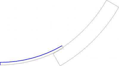
The principle of result polygon building is to build polygon by taking edges localized as in or on.

Generally, the principle is to take an edge in P1 with wanted loc and linking direct neighbour-edges (with correct loc) until closing a polygon. If not, using P2 edges to try to close polygon. The process is repeated until all edges with correct loc have been consumed.

The method in charge of that is INTERP_KERNEL::QuadraticPolygon::buildIntersectionPolygons.

Underlying algorithms

Absolute localization algorithm

This algorithm is called when splitting process has been done, and that we are sure that the edge is either fully in ,or fully on or fully out.

The principle chosen to know if an edge E is completely included in an any polygon P is to see if its barycenter B is inside this any polygon P. After, for each nodes $ P_i $ of polygon P we store angle in $[-\pi/2,\pi/2 ]$ that represents the slope of line $ (BP_i) $ .
Then a line L going through B with a slope being as far as possible from all slopes found above. Then the algorithm goes along L and number of times N it intersects non-tangentially the any polygon P.

If N is odd B (and then E) is IN. If N is even B (and then E) is OUT.

This computation is very expensive, that why some tricks as described in localization techniques are used to call as few as possible during intersecting process.

Intersection algorithms

The only mathematical intersections performed are edges intersections. The algorithms used are :

Lin-Lin intersection : http://mathworld.wolfram.com/Line-LineIntersection.html
Lin-Arc intersection : http://mathworld.wolfram.com/Circle-LineIntersection.html
Arc-Arc intersection : http://mathworld.wolfram.com/Circle-CircleIntersection.html

Other algorithms

As internal architecture is quite general, it is possible to have more than classical intersection on any polygons :

area computation is available.
perimeter computation.
Hydraulic diameter computation.

Usage

This intersector is usable standalone. To use a set of user friendly methods have been implemented.

INTERP_KERNEL::QuadraticPolygon::buildArcCirclePolygon method builds from a std::vector of INTERP_KERNEL::Node* V, an instance of QuadraticPolygon P. P will have $N_{edges} = V.size()/2$ edges. Quadratic edge $Edge_i i \in [0,N_{edges}-1]$ starts with node V[i], ends with node V[i+1] and has a middle in $V[i+N_{edge}]$ .
If start, end and middle nodes of edge are aligned by a precision specified by INTERP_KERNEL::QUADRATIC_PLANAR::setArcDetectionPrecision.
INTERP_KERNEL::QuadraticPolygon::buildLinearPolygon method builds from a std::vector of INTERP_KERNEL::Node* V, an instance of QuadraticPolygon P. P will have edges. Linear edge $Edge_i i \in [0,N_{edges}-1]$ starts with node V[i] and ends with node V[i+1].

The orientation of polygons (clockwise, inverse clockwise) impact computation only on the sign of areas. During intersection of 2 polygons their orientation can be different.

The usage is simple :

...
// defining a precision
INTERP_KERNEL::QUADRATIC_PLANAR::setPrecision(1e-5);
INTERP_KERNEL::QUADRATIC_PLANAR::setArcDetectionPrecision(1e-5);
//
INTERP_KERNEL::QuadraticPolygon *polygon1=...;
bool isQuadratic=...//Depends on the nature of your cell. If your cell is MED_QUAD8 or MED_TRIA6 for example isQuadratic=true.
const double *externalTabXCoords=...;
const double *externalTabYCoords=...;
std::vector<INTERP_KERNEL::Node *> nodes;
INTERP_KERNEL::QuadraticPolygon *polygon2=0;
for(int i=0;i<nbOfNodes;i++)
  nodes.push_back(new INTERP_KERNEL::Node(externalTabXCoords[i],externalTabYCoords[i]));// First param of Node constructor is its X-axis and the second its Y-axis.
if(isQuadratic)
  polygon2=INTERP_KERNEL::QuadraticPolygon::buildArcCirclePolygon(nodes);
else
  polygon2=INTERP_KERNEL::QuadraticPolygon::buildLinearPolygon(nodes);
//play with polygons
double intersection=polygon1->intersectWith(*polygon2);
double dhydPol1=polygon1->getHydraulicDiameter();
double areaPol1=polygon1->getAreaOfZone();
//clean-up
delete polygon1;
delete polygon2;
...

Example of result

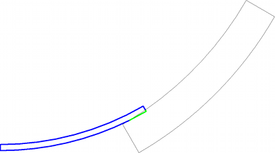
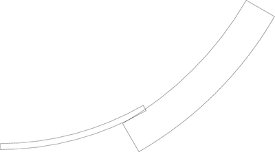
Here an example of 2 polygons. The left one P1 has 4 edges and the right one P2 has 4 edges too.

An example of intersection of 2 polygons.

After spliting process P1 has 6 edges and P2 has 6 edges too.

After spliting process two edges of P1 have been located has out.

Note: BLUE is for OUT, GREEN for IN and RED for ON.

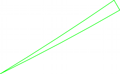
For each 6 edges locate them.

Result after locating phase.

Too finish closing polygons.

Close-up of final result after close polygons phase.

Note: The result polygon is constituted of 2 sub-edges coming from P1 and 1 sub-edge from P2 closing the polygon. For the 2 edges of P1 they are green because they are fully included in P2. Inversely, the only sub-edge coming from P2 is fully included in P1.